DSB-SC System Design and MATLAB Implementation
A double-sideband suppressed-carrier communication system design project. The design in this project are presented in three major parts, which are modulation, distortion and demodulation of the signal. The project can also be
Double-Sideband Suppressed-Carrier Communication System Implementation in Matlab. The DSB-SC system composed of:
- Modulation of a signal, which modulates the amplitude of the incoming signal
- Distortion of a signal when it passes through a communication channel
- Demodulation of a signal, which utilize the low-pass-filter. In which the final signal will form a scaled and distorted version of the original message signal.
Introduction to DSB-SC and design overview
Double-sideband suppressed-carrier (DSB-SC) transmission
Double Sideband Suppressed Carrier transmission is the transmission of a modulated wave, which only sidebands are transmitted through the communication system, while the carrier wave is being suppressed.
In example above, the frequency of message and carrier wave is 100Hz and 500Hz respectively and the amplitude of both is 1.
DSB-SC communication system design problem statement
Design a DSB-SC communication system following the diagram below
Given channel characteristic \(H(f)=e^{-2j\pi30t}+e^{-2j\pi5t}\)
Baseband signal for my DSB-SC system
Baseband message signal m(t) is composed with three frequencies, based on my last 3 digits of my student ID, which is 2021610064 (old)
\[m(t)=cos(2\pi100t)-\frac13cos(2\pi60t)+\frac15cos(2\pi4t)\]Overview of the system design
Introduction to the approach to the design of each part of the system, which each steps will be expand further in the next respective sections.
Message signal modulation
Generation of modulated message signal, m(t), with the carrier signal, resulting in a DSB-SC modulated waveform.
\[x(t)=m(t)\times c(t)\]Where x(t) is the output modulated signal, m(t) is the message signal, and the multiplying term, c(t) , is the carrier signal.
Channel distortion
Once the modulated signal pass through the Linear Time-Invariant communication channel, distortion will have effect on the passing signal, by the channel characteristic.
Demodulation of signal
Demodulated signal is the product of y(t) and the carrier signal.
\[v(t)=y(t)\times c(t)\]Where v(t) is the demodulated signal, y(t) is the modulated signal after being distorted through the communication channel.
Entering Low-Pass-Filter
Passes original message signals, with a frequency lower than the cutoff frequency and reduce the amplitude of carrier signals with frequencies higher than the cutoff frequency.
Resulting output signal
The resulting signal after the demodulation and the application of the Low pass filter, will be a scaled and distorted version of the message signal.
Note on graphical plots
The range of the time that use to scale the figures in time domain is from -0.1 to 0.1, with incrementation of \(1/f_s\), where \(f_s\) is the sampling frequency.
Modulated Signal Analysis
Baseband signal observation
Baseband signals are signals that occupied the range of frequencies, which has not been through the process of modulation.
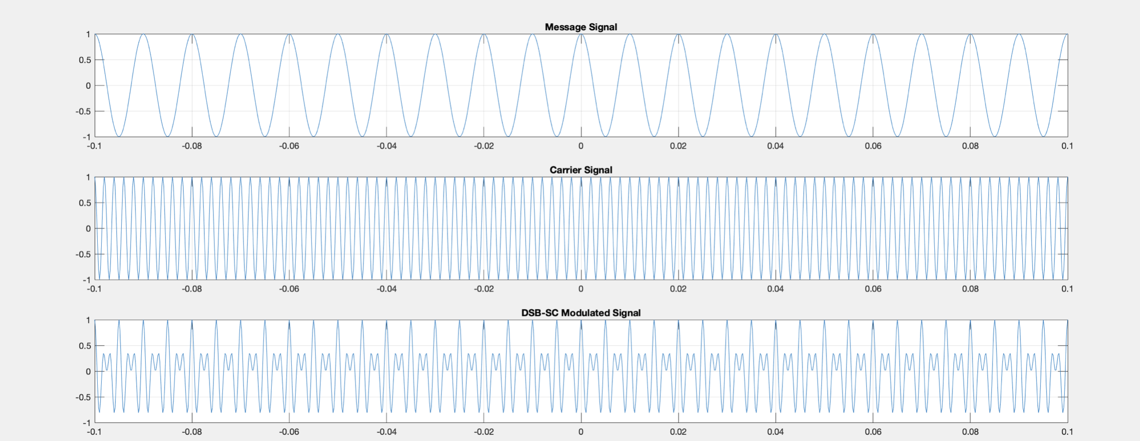
Message and Carrier signals
The message signal and the carrier signal, \(c(t)=A_ccos(2\pi f_ct)\) with carrier signal amplitude of 1 and frequency of 1kHz is plotted and shown below.
Fourier transform of Message signal
We can observe the frequency range of the message signal clearer in the frequency domain. As shown in figure 2.1.2, the frequencies are around at 4Hz, 60Hz and 100Hz, which represent the frequencies of the message.
Modulation of the Message signal
From modulated wave equation, we can get the modulated signal from the product of the message signal and the carrier signal. The plot of the signal after DSB-SC modulation is shown in figure below.
From the modulated signal, \(x(t)=m(t)\times c(t)\)
\[x(t)= (cos(2\pi100t)-\frac13cos(2\pi60t)+\frac15cos(2\pi4t))\times (cos(2\pi 1000t))\]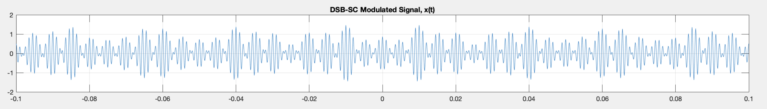
Fourier transform of modulated signal
If we take the Fourier transform of the modulated signal, it is apparent that the carrier signal component is being suppressed, as it isn’t visible in the output signal in frequency domain.
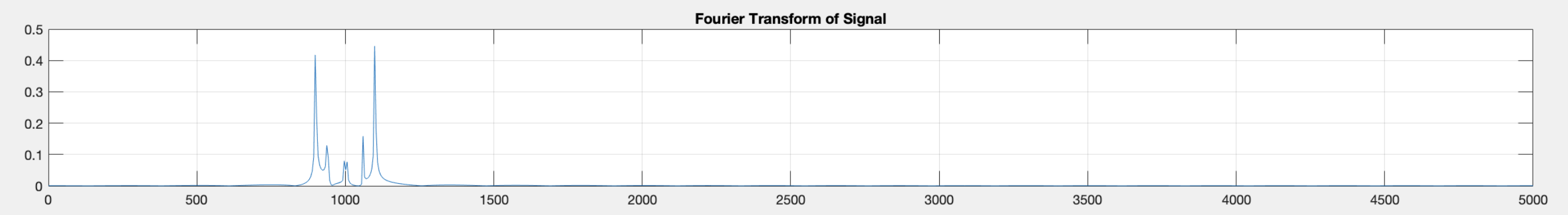
When the spectrum of the output signal is viewed. In figure above we see six peaks, the three peaks below 1kHz are the lower sideband and the three peaks above 1kHz are the upper sideband, but there is no peak at the 1kHz point, which denotes the frequency of the carrier, which has been suppressed.
Distortions in communication channel
Channel distortion in frequency domain
To get the signal y(t), with given channel characteristic H(f), we can convert x(t) to X(f), and use the converted signal to find Y(f) in frequency domain. Which lastly the signal can be convert back to time domain as y(t).
Convert x(t) to X(f) in frequency domain
We can take the Fourier transform of the signal x(t) to get X(f).
\[X(f)=\int_{-\infty}^{\infty} x(t)\ e^{-2\pi j t} \,dt\] \[X(f)=\int_{-\infty}^{\infty} (cos(2\pi100t)-\frac13cos(2\pi60t)+\frac15cos(2\pi4t))\times (cos(2\pi 1000t)) \cdot e^{-2\pi j t} \,dt\] \[\begin{align} {X(f)=} {\frac{1}{2} [\pi\delta(f-1800\pi)+\delta(f+1800\pi)]} - \\ {\frac{1}{6} [(\pi\delta(f-1880\pi)+\delta(f+1880\pi)]} + \\ {\frac{1}{10} [(\pi\delta(f-1992\pi)+\delta(f+1992\pi)]} + \\ {\frac{1}{10} [(\pi\delta(f-2008\pi)+\delta(f+2008\pi)]} - \\ {\frac{1}{6} [(\pi\delta(f-2120\pi)+\delta(f+2120\pi)]} + \\ {\frac{1}{2} [(\pi\delta(f-2200\pi)+\delta(f+2200\pi)]} \end{align}\]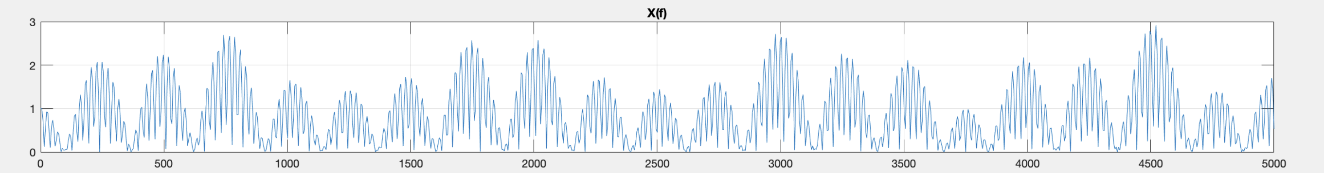
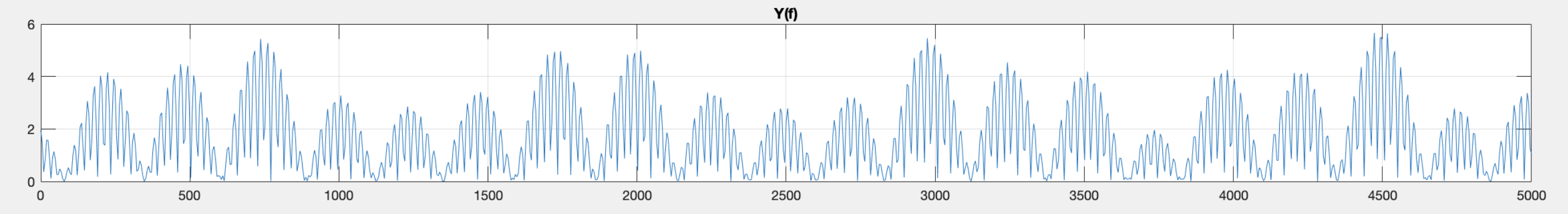
Apply Channel Distortion

Now that both of the channels characteristic and the modulated signal are in the frequency domain, the input-output relationship in frequency domain is given by \(Y(f) = H(f)X(f)\).
\[\begin{align} {Y(f)=} {X(f) H(f)} \end{align}\] \[\begin{align} {Y(f)=} \pi(\delta(f-1800\pi)+\delta(f+1800\pi))(1+1.1392e^{-14j})- \\ \pi(\delta(f-1880\pi)+\delta(f+1880\pi))(\frac{1}{3}+3.7972e^{-15j})+ \\ \pi(\delta(f-1992\pi)+\delta(f+1992\pi))(\frac{1}{5}+2.2783e^{-15j})+ \\ \pi(\delta(f-2008\pi)+\delta(f+2008\pi))(\frac{1}{5}+2.2783e^{-15j})- \\ \pi(\delta(f-2120\pi)+\delta(f+2120\pi))(\frac{1}{3}+3.7972e^{-15j})+ \\ \pi(\delta(f-2200\pi)+\delta(f+2200\pi))(1+1.1392e^{-14j}) \end{align}\]By multiply H(f), which is given by the channel characteristic equation and shown in figure 3.1.2 i. with X(f), the resulting signal will be Y(f) in the frequency domain
Conversion to Time Domain
Convert Y(f) bcak to y(t)
We can take the inverse Fourier transform to the signal Y(f) to get y(t), which is in the time domain again.
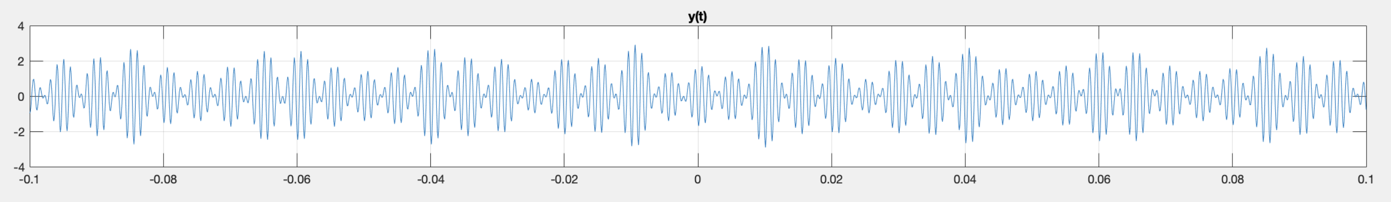
Demodulated signal analysis
Signal Demodulation
Demodulated signal
The first step of DSB-SC demodulation is done by multiplying the DSB-SC modulated signal with the carrier signal.
\[v(t)=y(t)\times c(t)\] \[\begin{align} {v(t)=} \frac{1}{2\pi}\big[ \pi(e^{-\pi t 1800 j}+e^{\pi t 1800 j})(1+1.1392e^{-14j})- \\ \pi(e^{-\pi t 1880 j}+e^{\pi t 1880 j})(\frac{1}{3}+3.7972e^{-15j})+ \\ \pi(e^{-\pi t 1992 j}+e^{\pi t 1992 j})(\frac{1}{5}+2.2783e^{-15j})+ \\ \pi(e^{-\pi t 2008 j}+e^{\pi t 2008 j})(\frac{1}{5}+2.2783e^{-15j})- \\ \pi(e^{-\pi t 2120 j}+e^{\pi t 2120 j})(\frac{1}{3}+3.7972e^{-15j})+ \\ \pi(e^{-\pi t 2200 j}+e^{\pi t 2200 j})(1+1.1392e^{-14j}) \big]\ cos(2\pi 1000t ) \end{align}\]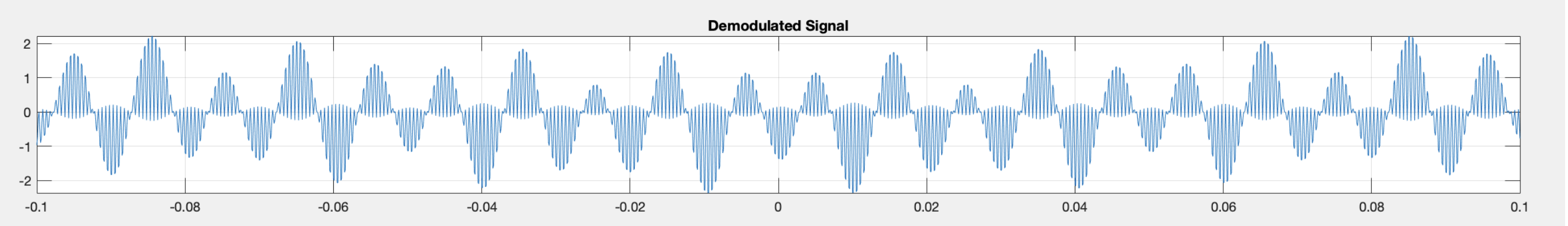
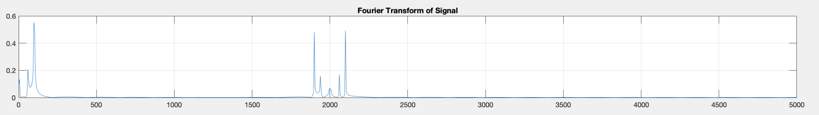
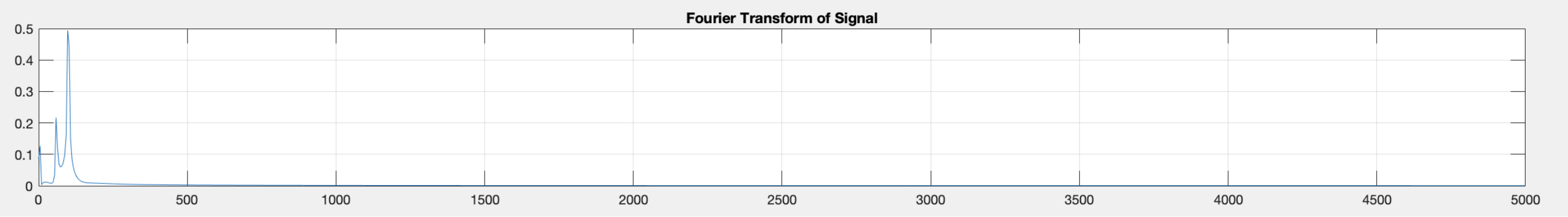
Fourier transform of demodulated signal
It is apparent in figure below, that there is 2 batches of frequencies along the frequency spectrum, which the lower frequency batch is the original message, while the higher are the DSB-SC modulated signal’s.
Low Pass Filter (LPF)
Application of Low pass filter
This demodulated signal is passed through a low pass filter to form a scaled version of the original message signal and for the signal to pass only the message signal.
Characteristic of signal after application of LPF
A low-pass filter or LPF passes signals with a frequency lower than the cutoff frequency and decrease the signal with frequencies higher than the cutoff frequency. Which means once the demodulated signal passes through the low pass filter, the higher frequency component, or the carrier’s frequency is removed, leaving just the original message.
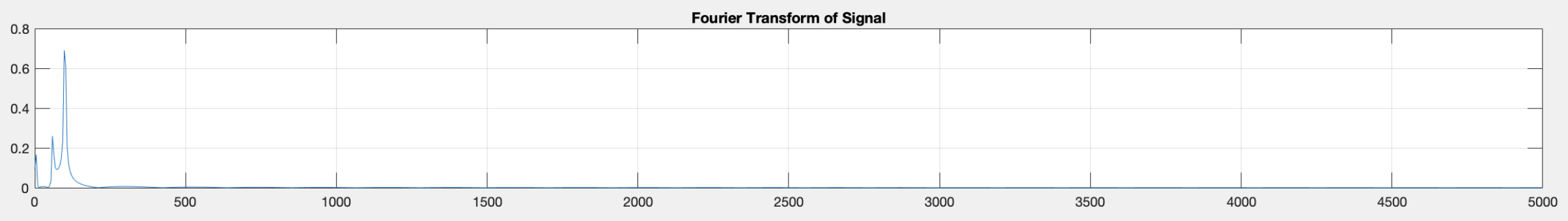
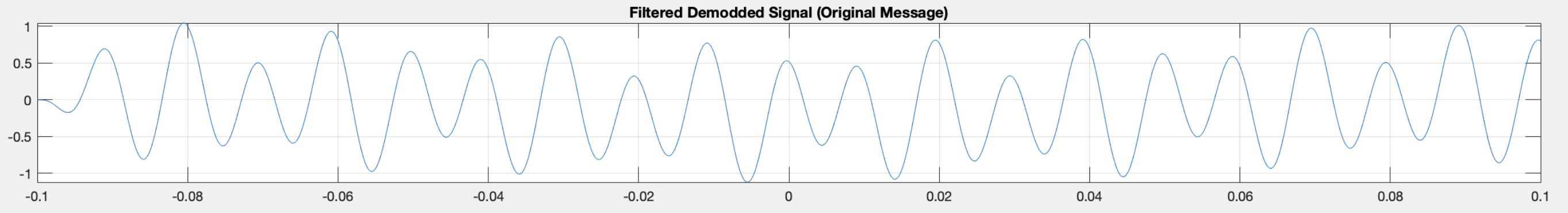
Fourier transform of signal after application of LPF
From the plot of figure below, the remaining batch of frequencies on the frequency spectrum is from only the message signal, hence, the demodulation of the signal.
Output signal result
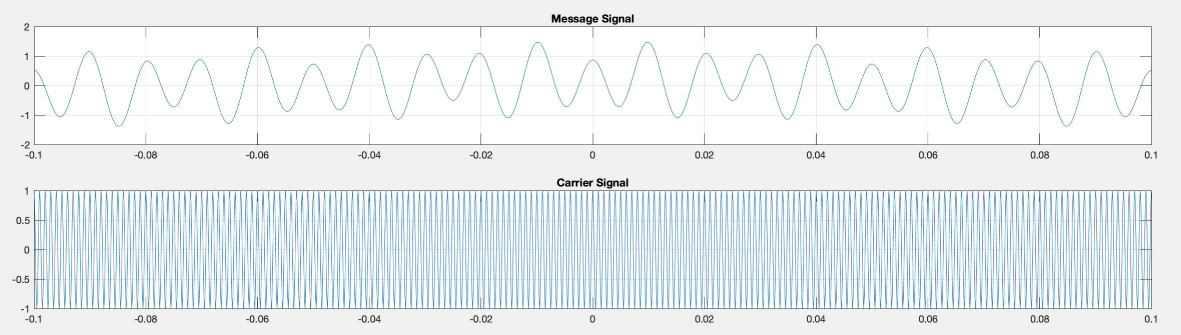
The resulting Filtered demodulated signal in time domain figure is the message signal that has been modulated, distorted through communication channel, demodulated and applied low pass filter. Which the signal presented in the said figure is the signal that the receiver will receive.
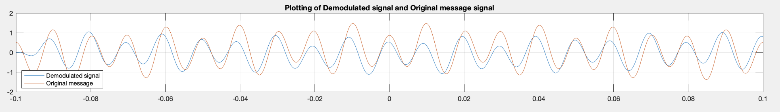
Original message comparison in time domain
By comparing the final resulting signal and the original message signal in the time domain in figure below. The following observations can be make:
- The final resulting signal after modulation, distortion, demodulation and filtration is a scaled and distorted version of the original message signal.
- The amplitude of the demodulated (final) signal appears to be slightly lower than the amplitude of the original message signal.
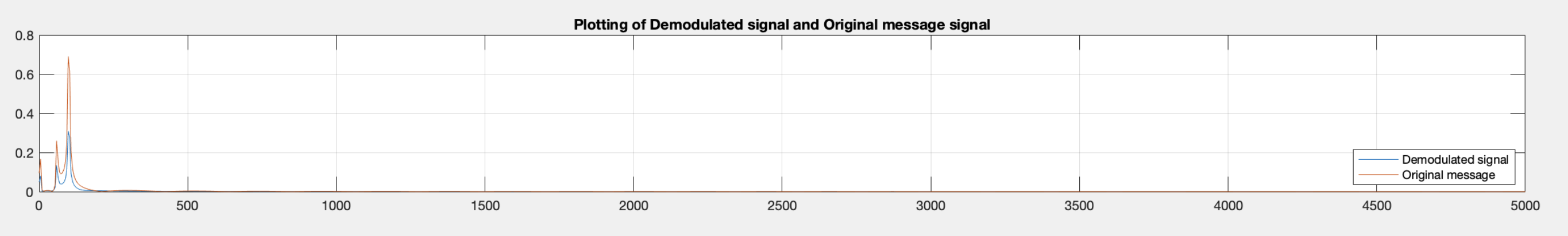
Original message comparison in frequency domain
And by comparing the final resulting signal and the original message signal in the frequency domain in figure below. We can observe that:
- The amplitude of the demodulated signal has been attenuated and scaled down from the original message signal.
- However, the distribution of frequencies of the demodulated signal remains the same as the original message, which are around 4, 60 and 100 Hz on the frequency spectrum.
Conclusions
Given a baseband signal, with no prior modulation, with frequency respecting to student’s ID number. We can design a DSB-SC communication system. In order of modulation, channel distortion, demodulation and low pass filter.
A message signal can be modify by multiplying with a carrier signal. This type of amplitude modulation is called “Double-sideband suppressed-carrier” or DSB-SC modulation. The signal that has been modulated, are affected with channel distortions, which are distinguish by the channel characteristics, and are differs from channels to channels.
The demodulation of a signal can be obtain by the product of the modulated signal and the carrier signal. After getting the product, the signal is now demodulated, but with the carrier signal’s frequency included. In order to attenuate the carrier frequency, we can apply low pass filter to the signal. The original message will be the only thing that’s left in the output signal, while the carrier signal component is suppressed.
The final signal will output a scaled and distorted version of the original message signal.