Crime Data Analysis and Trend Classsification Using Python
As crime rate spikes during the last few years throughout USA, I made the decision to take data from one of the most populated city in the USA and take a closer look on the criminal activity itself in order to gain insights to the climate of the crime and it’s surrounding factors, visualize if any patterns occurred. And how the factors all related or unrelated to one another, how they can be use to correlate the occurred crime to other factors, which ultimately can help us predict and determine future circumstances of the crime in the area.
0 Project Repository
You can check out the code of this project here!
1 Problem statement
1.1 What is a crime?
A crime is an act or instance that is considered to be against the morals or laws of society. A crime can also mean illegal activity in general or a frequent committing of such activity. Crime can also mean a repeated or frequent performing of illegal acts. And crime can be used more generally to refer to any offense.
1.2 Problem
As stated above:
As crime rate spikes during the last few years throughout USA, I made the decision to take data from one of the most populated city in the USA and take a closer look on the criminal activity itself in order to gain insights to the climate of the crime and it’s surrounding factors, visualize if any patterns occurred. And how the factors all related or unrelated to one another, how they can be use to correlate the occurred crime to other factors, which ultimately can help us predict and determine future circumstances of the crime in the area.
1.3 Proposed Solution
Firstly, we need to fully understand the data and how the features and factors correlate. To do that, we can implement several libraries to manipulate the data and visualize them for ease of analysis.
Using EDA methodologies to explore insights and topics according to contexts gathered from the data and find the patterns in order to gain insights of the relation between several factors and occurrences.
In order to predict crimes that hasn’t occurred yet, we can implement several Supervised Classification Machine Learning methodologies. With several models created, we can determine the most optimal model and further analyze the factors and parameters in order to fully optimize the method.
2 Data & Preparation
Crime in Los Angeles: Crime data from 2010 through September 2017
This dataset reflects incidents of crime in the City of Los Angeles dating back to 2010. This data is transcribed from original crime reports that are typed on paper and therefore there may be some inaccuracies within the data. Some location fields with missing data are noted as (0°, 0°). Address fields are only provided to the nearest hundred block in order to maintain privacy.
Column Description
26 columns including: DR Number, Date Reported, Date Occurred, Time Occurred, Area ID, Area Name, Reporting District, Crime Code, Crime Code Description, MO Codes, Victim Age, Victim Sex, Victim Descent, Premise Code, Premise Description, Weapon Used Code, Weapon Description, Status Code, Status Description, Crime Code 1, Crime Code 2, Crime Code 3, Crime Code 4, Address, Cross Street, Location
DR Number: Division of Records Number: Official file number made up of a 2 digit year, area ID, and 5 digits.
Date Reported / Occurred: Date which crime was reported/occurred.
Time Reported / Occurred: Time which crime was reported/occurred.
Area ID: The LAPD has 21 Community Police Stations referred to as Geographic Areas within the department. These Geographic Areas are sequentially numbered from 1-21.
Area Name: The 21 Geographic Areas or Patrol Divisions are also given a name designation that references a landmark or the surrounding community that it is responsible for. For example 77th Street Division is located at the intersection of South Broadway and 77th Street, serving neighborhoods in South Los Angeles.
Reporting District: A four-digit code that represents a sub-area within a Geographic Area. All crime records reference the “RD” that it occurred in for statistical comparisons.
Crime Code: Indicates the crime committed. (Same as Crime Code 1)
Crime Code Description: Defines the Crime Code provided.
MO Codes: Modus Operandi: Activities associated with the suspect in commission of the crime.
Victim Age: Two character numeric.
Victim Sex: F - Female M - Male X - Unknown.
Victim Descent: Descent Code: A - Other Asian B - Black C - Chinese D - Cambodian F - Filipino G - Guamanian H - Hispanic/Latin/Mexican I - American Indian/Alaskan Native J - Japanese K - Korean L - Laotian O - Other P - Pacific Islander S - Samoan U - Hawaiian V - Vietnamese W - White X - Unknown Z - Asian Indian.
Premise Code: The type of structure, vehicle, or location where the crime took place.
Premise Description: Defines the Premise Code provided.
Weapon Used Coded: The type of weapon used in the crime.
Weapon Description: Defines the Weapon Used Code provided.
Status: Status of the case. (IC is the default).
Status Description: Defines the Status Code provided.
Crime Code 1: Indicates the crime committed. Crime Code 1 is the primary and most serious one. Crime Code 2, 3, and 4 are respectively less serious offenses. Lower crime class numbers are more serious.
Crime Code 2: May contain a code for an additional crime, less serious than Crime Code 1.
Crime Code 3: May contain a code for an additional crime, less serious than Crime Code 1.
Crime Code 4: May contain a code for an additional crime, less serious than Crime Code 1.
Cross Street: Cross Street of rounded Address.
Location: Street address of crime incident rounded to the nearest hundred block to maintain anonymity.
Acknowledgements
This dataset was released by the City of Los Angeles. Last update 2018
2.2 Imports Libraries and Reading Data
In order to manipulate and analyze the data, necessary libraries are need to be imported.
import matplotlib.pyplot as plt
import numpy as np
import pandas as pd
import datetime as dt
import seaborn as sns
from pylab import rcParams
%matplotlib inline
rcParams["figure.figsize"] = 12, 8
After that, by using read_csv() from pandas, and routing the path to the dataset, we can now begin our manipulations and analysis.
crime = pd.read_csv(path)
2.3 Data Preparation
After importing the data, I noticed that the date and time is not in the most optimal format, so I reformat the feature and then reassign them in their original column.
try:
    date_reported = [dt.datetime.strptime(d, "%m/%d/%Y").date() for d in crime["Date Reported"]]
except:
    print("Already converted Date Reported")

try:
    date_occurred = [dt.datetime.strptime(d, "%m/%d/%Y").date() for d in crime["Date Occurred"]]
except:
    print("Already converted Date Occurred")

crime["Date Reported"] = np.array(date_reported)
crime["Date Occurred"] = np.array(date_occurred)
Afterwards, in order to visualize the properties properly, I make lists of days, months, and years for reported/occurred from datetime objects and then make a new column for each new features.
day_reported = [d.isoweekday() for d in crime["Date Reported"]]
mon_reported = [d.month for d in crime["Date Reported"]]
year_reported = [d.year for d in crime["Date Reported"]]

crime["Day Reported"] = np.array(day_reported)
crime["Month Reported"] = np.array(mon_reported)
crime["Year Reported"] = np.array(year_reported)
With this, we are now ready to visualize and analyze our data.
3 Data Visualization
3.1 Shape
There are total of 1584316 items with 26 columns for each items.
The columns are being: DR Number, Date Reported, Date Occurred, Time Occurred, Area ID, Area Name, Reporting District, Crime Code, Crime Code Description, MO Codes, Victim Age, Victim Sex, Victim Descent, Premise Code, Premise Description, Weapon Used Code, Weapon Description, Status Code, Status Description, Crime Code 1, Crime Code 2, Crime Code 3, Crime Code 4, Address, Cross Street, Location.
3.2 Date, Time and Period of crime reported and occurred
The graphs in the following section uses seaborn’s barplot() to visualize.
sns.barplot()
Crime reported and occurred - by day
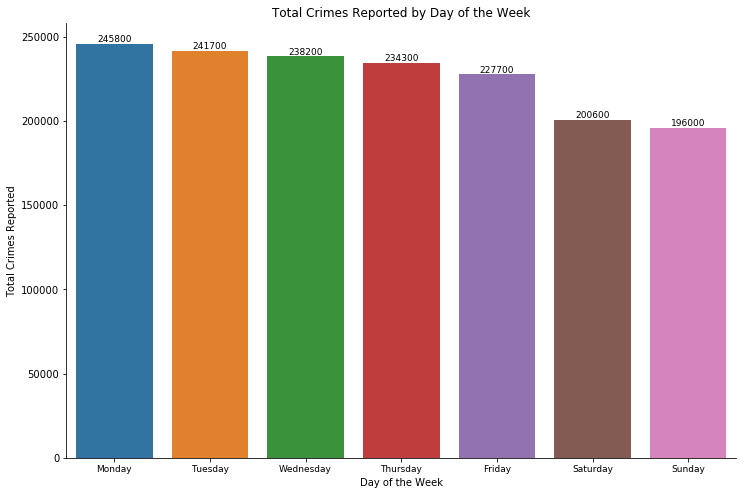
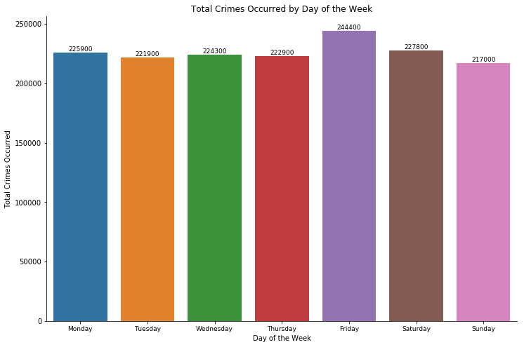
We can gather by the 2 graphs that:
- Saturday and Sunday are the 2 days that crimes are least likely to be reported, this is inarguably because, they are weekends. During weekends, people are less likely to be active, including both the criminal act and the duty of reporting the crime.
- Friday is the day that crime is most likely to occur. My analysis on this fact is that on Friday, more people will be out in the city and enjoying the night life, which mean, there will be more victims of petty crimes such as stealing or robbery for that day.
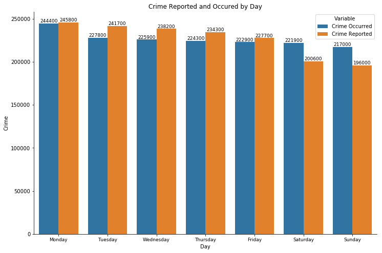
Comparison of crime reported and occurred - by day
There are significantly more crimes occurs during the weekend, yet fewer crimes reported on Saturday and Sunday. The reason is possibly be aligned with the above individual analysis.
Crime reported and occurred- by month
July and August seems to be the months that have the most crime in term of reported crimes and occurred crimes.
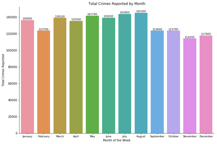
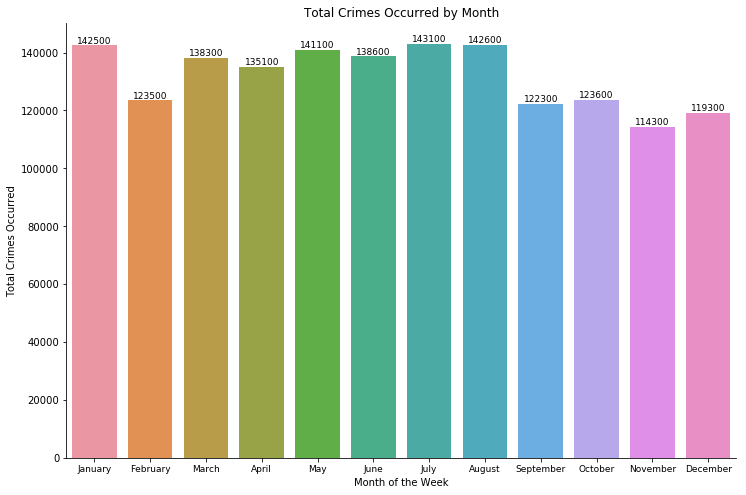
Comparison of crime reported and occurred - by month
We can see that months such as January or August, which have 31 days generally have more crimes than the ones with fewer days.
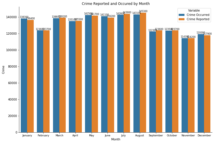
The last 4 months of the graph have a significant decrease in the number of crimes both reported and occurred, this is because the crime dataset is only up to September, which explains the lack of both reports and occurrences during those months.
Crime Reported and occurred - by year
For crime reported and occurred by year, I used normal plot, to show a clear increase/decrease of the values each year
plt.plot()
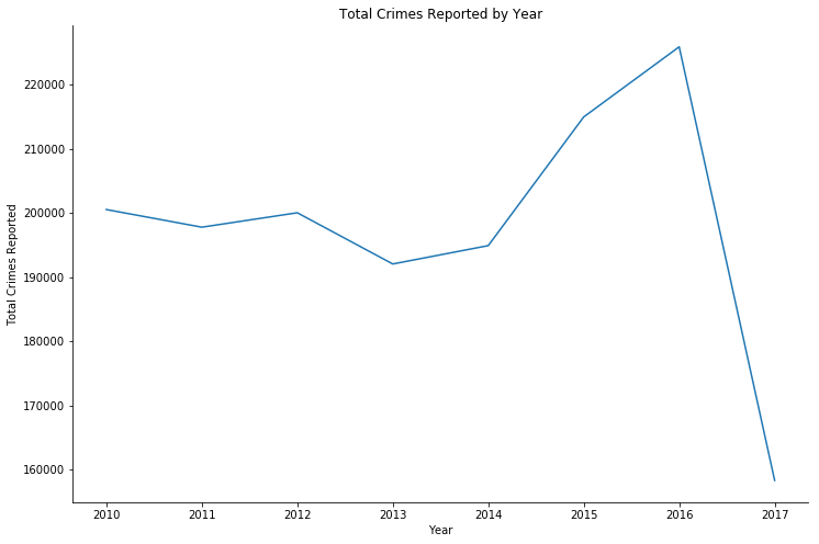
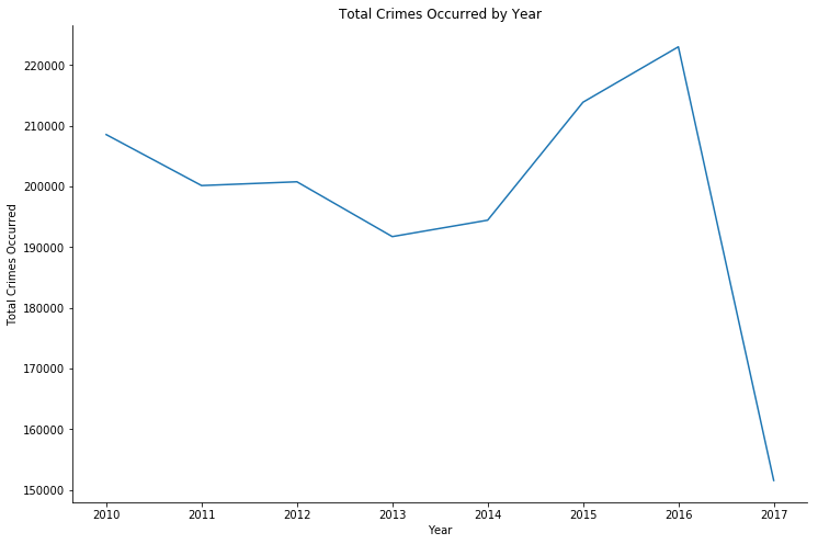
Both reported and occurred crimes has been significantly increases.
Comparison of crime reported and occurred - by year
The increases of both reported and occurred of the last 3 years are clearly represented in the comparison bar graph below.
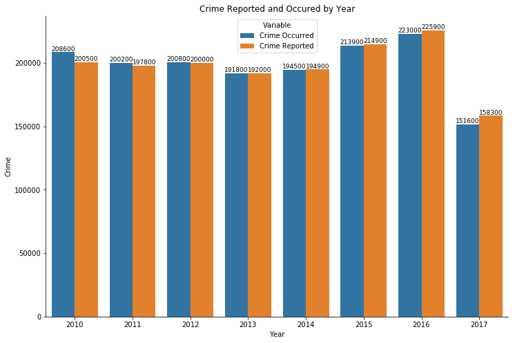
And again, the dataset is only up to date as of September 2017, hence the lack of both crime reported and occurred during the year 2017.
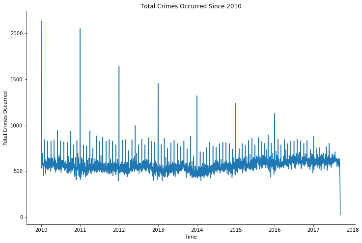
Crime reported and occurred - over time (chronologically)
For chronologically represent the crimes reported and occurred, I used normal plt.plot().
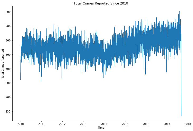
There is an upward trend of increasing crime reported over the last 3 years, proves the correlation to the last point. Which again, causes by the limitation of the dataset, which only contains data up to September 2017.
The spikes within crime occurrence dates within each years is an unknown date of the crime. And these crimes are such as “Identity Theft” because it is not possible in most case to pinpoint the exact date the crime occurred. So, all crimes with unknown occurring date are all attributed to a specific date within the year of occurrence.
Crime reported and occurred - over month and year
Again, I used the plt.plot() for a clear visualization of the trends in the following graphs.
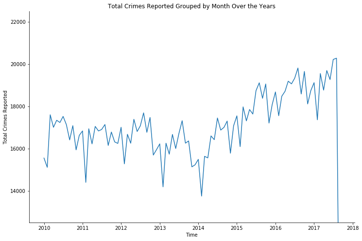
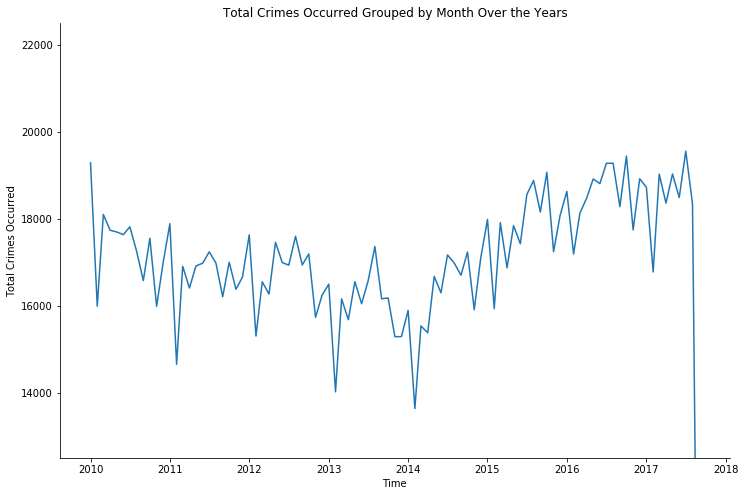
We then see the upward trend again for the last 3 years, which correlate to the graph in the last section.
And the sudden sharp decrease at the end attributes to the limitation of the dataset once more.
Crime throughout the day
Below graphs are visualizations of crimes that occurs through out the day, and the right graph is from investigate by hour.
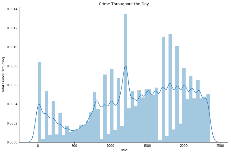
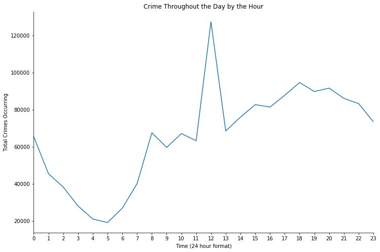
We can see clearly that both of the graphs suggested that there is a surge of crimes occurring at 12PM, which is an interesting point for investigation.
Which the analysis of what happened at the time can be investigate below in the next section (section 4.6).
All the date time related findings that we have observed so far, mostly is bounded by the limitation of the dataset itself, which capped off in September 2017, which is why we will explore this gap in data later in section 4.8.
3.3 Area name
For this section, a bar plot would be most optimal to visualize the crimes that has occurred in each area.
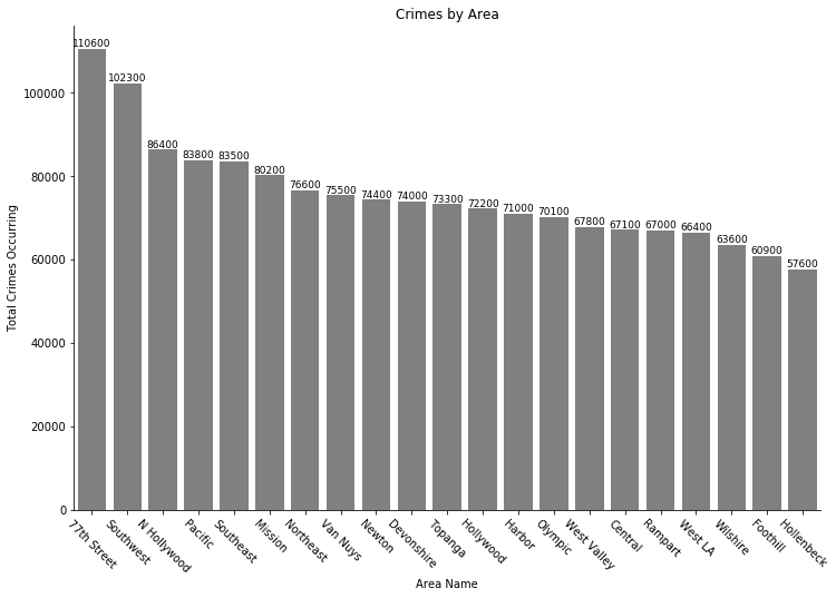
There are twice as much crimes in the 77th Street Area than Hollenbeck, which is interesting because of the population and square miles ratio.
- 77th Street: Approximately 175,000 population and 11.9 square miles.
- Hollenbeck: Approximately 200,000 population and 15.2 square miles.
This will also be further investigate in the further section (section 4.5).
3.3 Crime code and MO codes
3.3.1 Crime Codes

Battery leads the crime chart with a difference of at least 10% from the next crimes, Burglary from Vehicle & Stolen Vehicle.
This is just the first top 20 crimes that has been committed.
3.3.2 MO Codes
The word “modus operandi” is a Latin term that refers to a person’s or a group’s usual mode of operation, which is recognizable as a pattern. A modus operandi (abbreviated “M.O.”) is a term used to describe criminal behavior and is frequently utilized by professionals to avoid future crimes. Modi operandi can evolve throughout time, particularly in response to new experiences and shifting values.
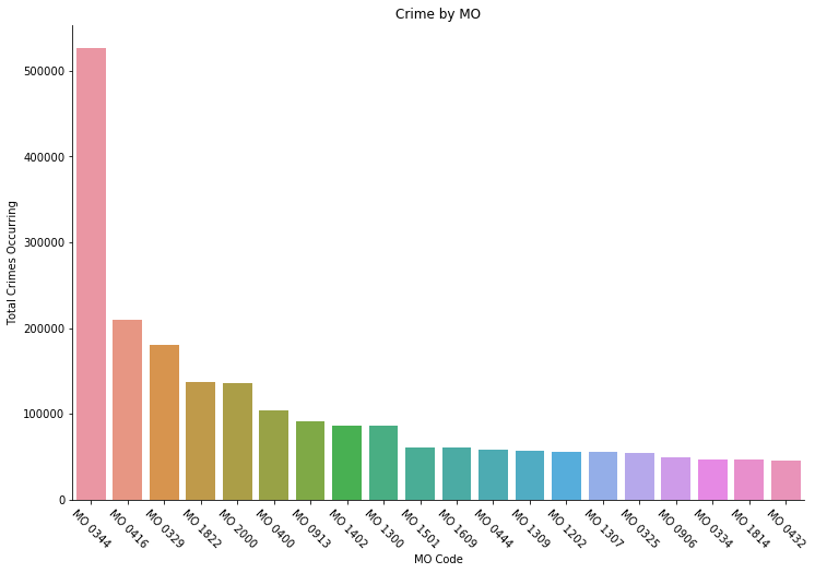
Notable codes:
- MO 0344: Removes victim property
- MO 0416: Hit with weapon
- MO 0329: Vandalized
- MO 1822: Stranger
- MO 2000: Domestic violence
3.4 Victim data
3.4.1 Victim Age
Basic information about victim’s age can be gathered as below:
| Mean | 35.934195 |
|---|---|
| STD | 16.811559 |
| Min | 10.000000 |
| 1st Quartile | 23.000000 |
| 2nd Quartile | 34.000000 |
| 3rd Quartile | 48.000000 |
| Max | 99.000000 |
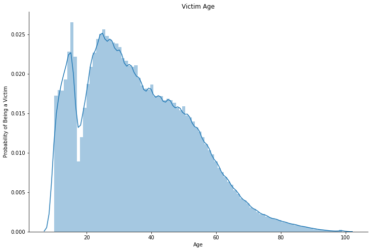
Mean of the victims are 35, and is supported by a median of 34.
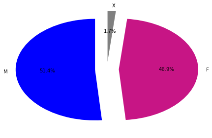
3.4.2 Victim Sex
The demographics of victim’s sex can be gathered below:
| Male | 739581 |
|---|---|
| Female | 675402 |
| Other | 24080 |
| N/A | 54 |
I use pie chart to visualize the data in this case:
The sex of the victim are distributed as 51.4% being male, 46.9% being women, and 1.7% of other
3.4.3 Victim Descent
Before visualizing the data, some preparation is to be done, namely renaming the abbreviations to the whole description.
Victims_bg = {
    "A": "Other Asian",
   .
   .
   .
    "Z": "Asian Indian"
}
crime["Victim Descent"] = crime["Victim Descent"].map(Victims_bg)
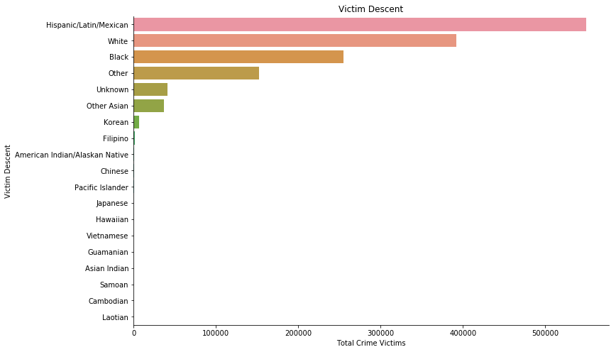
Hispanic/ Latin/ Mexican has been the crime victims of the most crime. While there are 7000 Korean crime victims and only 2000 Filipino crime victims in the last 5 years.
3.5 Premise Description
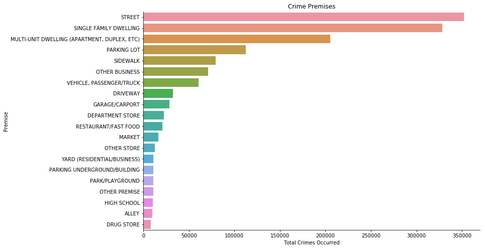
The top premise for crime committed is on the street and the runner-up is the single family dwelling. More analysis will be done in section 4.3.
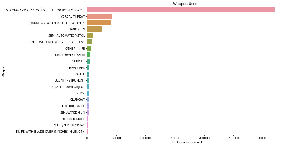
3.6 Weapon Description
Before visualizing weapon data, we can check for missing weapon data, if any.
missvals = crime["Weapon Description"].isnull().sum()
print("There are {} missing values".format(missvals))
There are 1509560 missing values.
We can assume that missing weapon values (Na) are either true missing, or no weapon was used.
3.7 Status Description
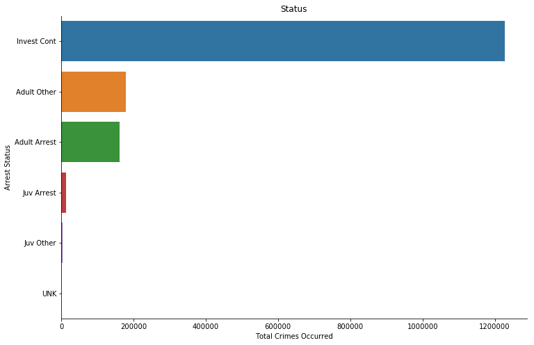
From the visualization above, we can investigate that there are over 6 times more of the ongoing investigations than adult arrests.
3.8 Crime Code
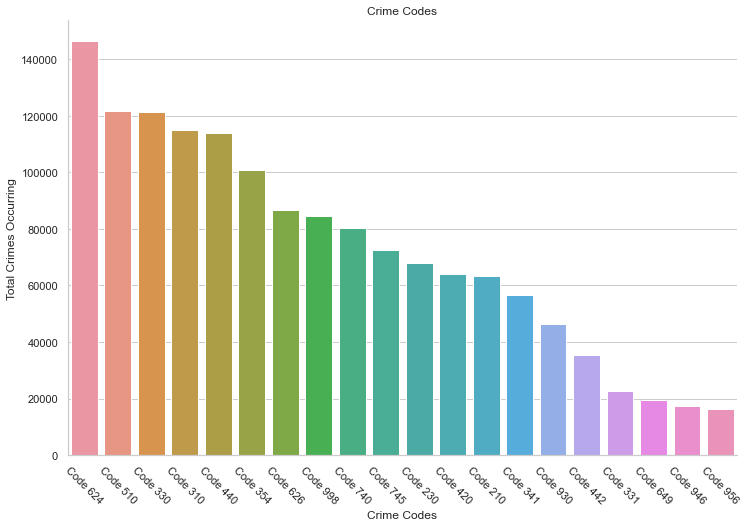
The most prominent crime is crime code 624, which is Battery and Simple Assault. And the follow up is crime code 510, which can be explain as Vehicles related crime. Both of the crimes are very likely to occur in real life.
4 Exploratory Data Analysis & Contextual Insights
4.1 Finding the relationship between gender and crime type
First we group the crime code description and the gender of the victim.
| Crime Code Description | Victim Gender | Count | |
|---|---|---|---|
| 0 | ASSAULT WITH DEADLY WEAPON, AGGRAVATED ASSAULT | F | 18422 |
| 1 | ASSAULT WITH DEADLY WEAPON, AGGRAVATED ASSAULT | M | 49034 |
| 2 | BATTERY - SIMPLE ASSAULT | F | 77588 |
| 3 | BATTERY - SIMPLE ASSAULT | M | 68070 |
| 4 | BURGLARY | F | 46685 |
| 5 | BURGLARY | M | 65197 |
| 6 | BURGLARY FROM VEHICLE | F | 54761 |
| 7 | BURGLARY FROM VEHICLE | M | 66187 |
| 8 | INTIMATE PARTNER - SIMPLE ASSAULT | F | 69360 |
| 9 | INTIMATE PARTNER - SIMPLE ASSAULT | M | 16524 |
| 10 | ROBBERY | F | 19008 |
| 11 | ROBBERY | M | 42988 |
| 12 | THEFT OF IDENTITY | F | 50767 |
| 13 | THEFT OF IDENTITY | M | 49523 |
| 14 | THEFT PLAIN - PETTY ($950 & UNDER) | F | 50000 |
| 15 | THEFT PLAIN - PETTY ($950 & UNDER) | M | 60692 |
| 16 | VANDALISM - FELONY ($400 & OVER, ALL CHURCH VA… | F | 31392 |
| 17 | VANDALISM - FELONY ($400 & OVER, ALL CHURCH VA… | M | 45523 |
| 18 | VANDALISM - MISDEAMEANOR ($399 OR UNDER) | F | 32982 |
| 19 | VANDALISM - MISDEAMEANOR ($399 OR UNDER) | M | 36914 |
The visualization can be observe below:
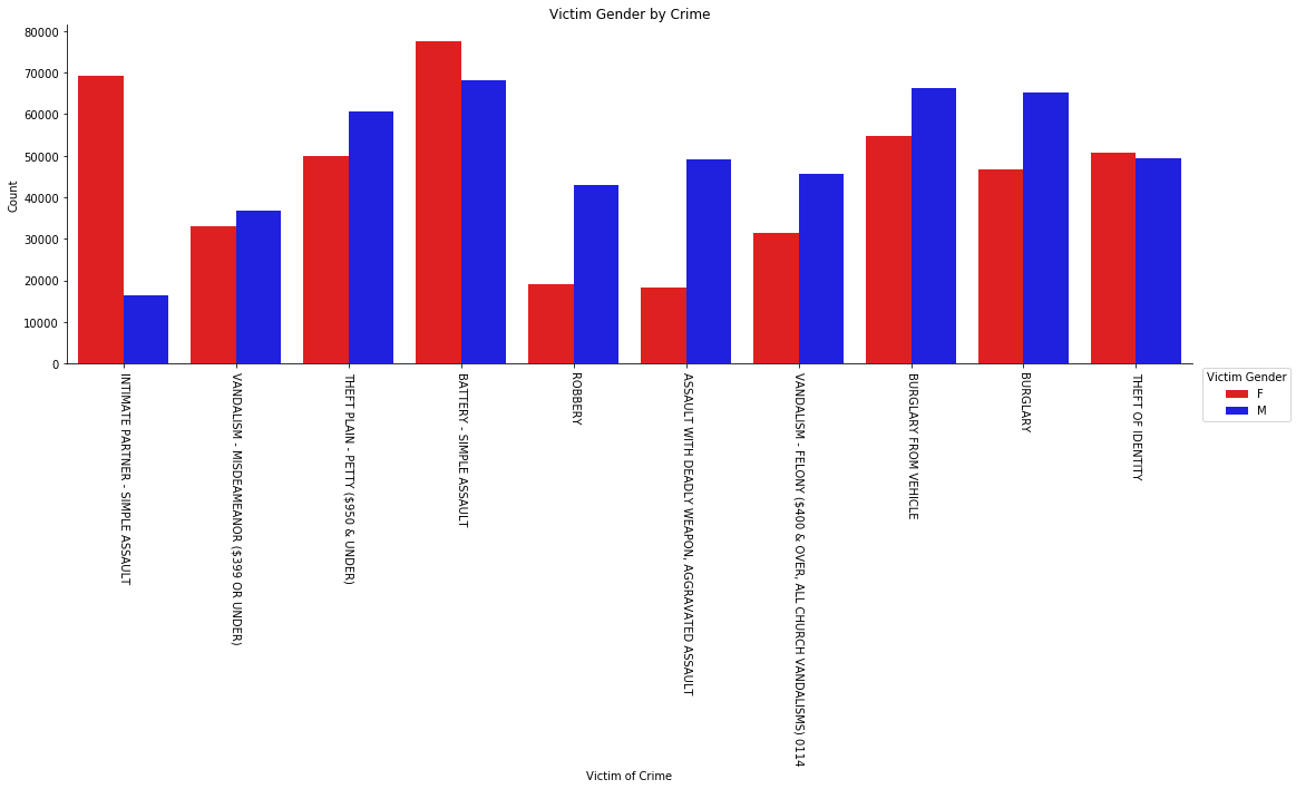
From the visualization, we can gather that:
- Vandalism (misdemeanor) and identity theft have a very close gender distribution for the respective crimes.
- Intimate partner sexual assault & Battery simple assault are the two crimes that women victims are more often are, which denotes the common occurrences of domestic violence that is still a common thing in the present, which is already more than a reason to fight for gender equality.
- It is because there are more cars owned by males than females, that the crime such as burglary and vehicle stolen related crime has more male victim than women victims.
4.2 Gun crime and correlated hour of occurrence
By filtering only rows with Hand guns or Semi-automatic pistols (by equal to), and group by Guns Only and Hour Occurred, we can observe the following:
crime["Guns Only"] = crime["Weapon Description"][(crime["Weapon Description"] == "HAND GUN") |
                                                 (crime["Weapon Description"] == "SEMI-AUTOMATIC PISTOL"
cc_gender = crime.groupby(["Hour Occurred", "Guns Only"]).size().reset_index(name="Count")
| last 6 items | Hour Occurred | Guns Only | Count |
|---|---|---|---|
| 42 | 21 | HAND GUN | 2066 |
| 43 | 21 | SEMI-AUTOMATIC PISTOL | 753 |
| 44 | 22 | HAND GUN | 1932 |
| 45 | 22 | SEMI-AUTOMATIC PISTOL | 690 |
| 46 | 23 | HAND GUN | 1837 |
| 47 | 23 | SEMI-AUTOMATIC PISTOL | 711 |
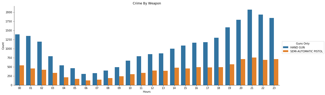
From the visualization above, we can observe that firearm activities generally occur at night, between 7pm and before midnight, from both handgun and semi-automatic pistols.
4.3 Premise of hour of occurrence and type of crime
Top 5 premises
| Street | 352160 |
|---|---|
| Single Family Dwelling | 328198 |
| Multi-Unit Dwelling | 204980 |
| Parking Lot | 112576 |
| Sidewalk | 79247 |
Hours of occurrence
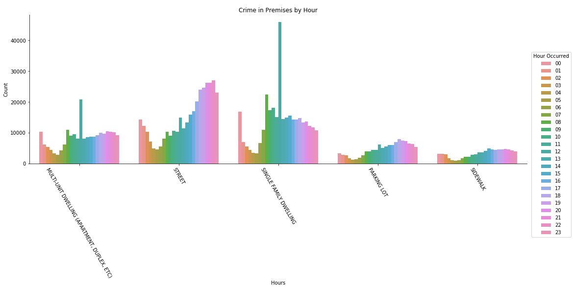
From the visualization above, we gather that:
- A prominent observation we can make of this graph is that the streets are generally less safe at night, and so is other crimes in the top 5 premises.
- In the single family dwellings, we can observe that there is a surge of crime again at12PM, which will be covered in section 4.6.
Type of crime
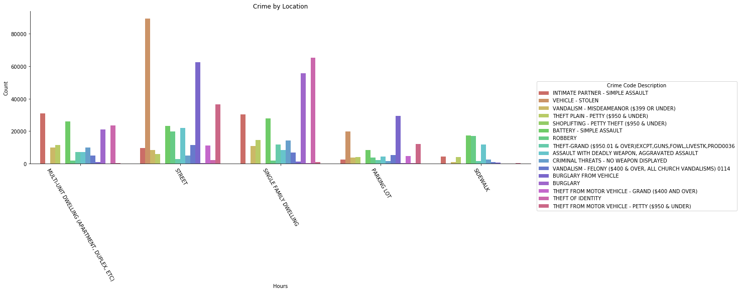
It is interesting to see that with the same amount of intimate partner sexual assault in multi-units and single family dwelling, the difference in identity theft and burglary is so significant.
Another thing is that vehicles are stolen four times more often in the street compared to the parking lot.
4.4 Juvenile arrests
I create and fill a new dataframe with only juvenile arrests.
crimejuv = crime.loc[crime["Status Description"].isin(["Juv Arrest"])]
It is easier to explore the data according to juvenile criteria by focusing on the victim of the said crimes .
First off, we can explore the age distribution of the victims of juvenile crimes for some basic understanding, and finding patterns.
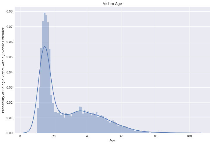
From the distribution graph above, we can observe that the Victim of the juvenile offenders tends to be between 10 to 20 years old.
Next, we would like to explore what crimes does the juvenile arrests committed. By plotting top 10 types of crime committed by a juvenile below.
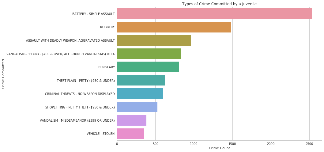
Battery and simple assault takes the lead to be the top type of crime juvenile arrest committed. Which on the contrary to the expected crime, which is vandalism or shoplifting. Which the data tells us that kids at younger age can lean towards violence. This might comes from several factors such as family, environment, influences of other media.
Now we have a basic understanding of the victims and the crime that committed by juvenile arrests. We would then like to explore more on the premise of the juvenile crime itself.
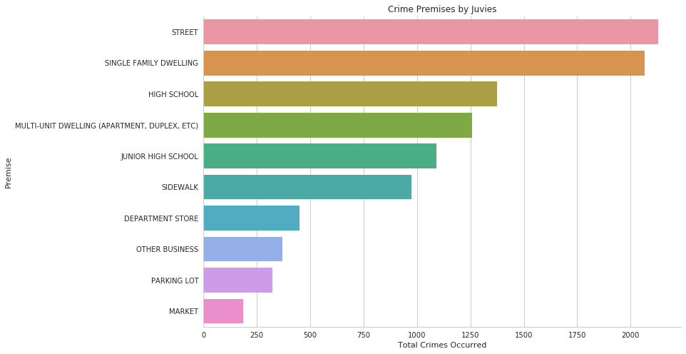
It’s difficult to say if single-family households have more children than multi-unit dwellings, or whether children in single-family dwellings are more likely to commit crimes than children in multi-unit dwellings. Whichever the case is, there is another surprising observation which can be depicted from the graph, which is: there are nearly equal amounts of juvenile crimes committed on the street as in a single family dwelling.
Lastly, we can explore the date and time of when the juvenile arrests committed the crime. First off, we are going to observe the crime by day of the week below.
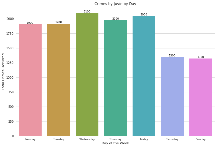
The most prominent take-away from the graph is that the crimes occur on weekdays since most juveniles are spending time with their family on the weekends.
Now we can observe the juvenile crime by the hour.
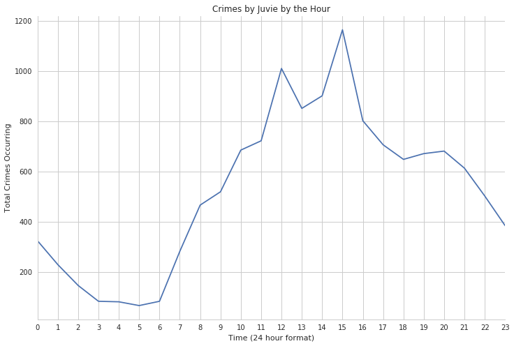
The take-away here is that juvenile crimes peaked between 12PM and 4 PM, which is also a school lunch hour, with the peak being at 3PM, as the time right after the school ends
We now understand a lot more regarding the crimes committed by juveniles, the next course of action regarding this topic that I want to suggest everyone to do is: look into these insights and find a way to reduce the future number of juvenile crime, and make a better, safer space for every children everywhere, not just in Los Angeles.
4.5 Difference of most dangerous and safest neighborhood by hour
As stated in the area section above, we are now going to observe the differences between the 2 safest and the most dangerous area respectively.
To do this, I take the max and min value of crimes occurring by Area, the safest and the most dangerous, which is Hollenbeck and 77th Street respectively. And group them by counts.
crime["Dang and Safe Area"] = crime["Area Name"][(crime["Area Name"] == "77th Street") |
                                           (crime["Area Name"] == "Hollenbeck")]
areahour = crime.groupby(["Dang and Safe Area", "Hour Occurred"]).size().reset_index(name="Count")
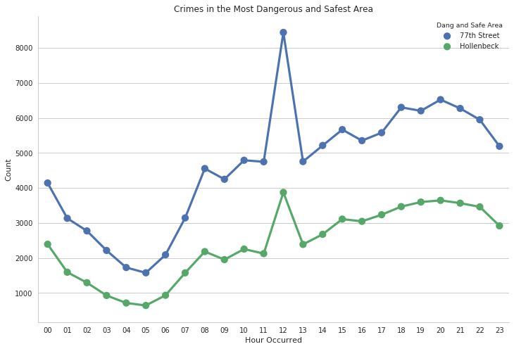
Hollenbeck has 13150 population per square mile
While 77th Street has 14700 population per square mile.
The population in 77th Street is dense and close in ratio of that with the Hollenbeck, the double in crime rate is surprisingly too significant. But this could also be missing the point of, what if these crimes were committed by someone not residing in the 77th Street.
4.6 Crime Surge at 12PM
As the visualize section above, there is a significant surge in crime during the hour of 12PM, which we will dive into understanding the root of these surges.
Firstly, I filter the data for only 12PM, and then take only the first top 6 crimes and top 6 premises, as a prepared data to be plot in a heatmap diagram.
crimenoon = crime.loc[crime["Hour Occurred"].isin(["12"])]
top6crimes = crimenoon["Crime Code Description"].value_counts().head(6).index
crimenoon = crimenoon.loc[crimenoon["Crime Code Description"].isin(top6crimes)]
top6premises = crimenoon["Premise Description"].value_counts().head(6).index
crimenoon = crimenoon.loc[crimenoon["Premise Description"].isin(top6premises)]

ccpremnoon = crimenoon.groupby(["Crime Code Description", "Premise Description"]).size().reset_index(name="Count")
ccpremise = ccpremnoon.pivot("Crime Code Description", "Premise Description", "Count")
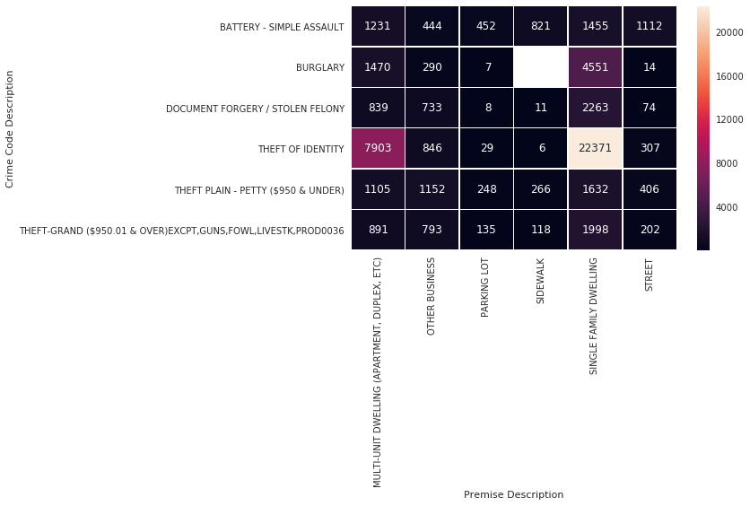
From the heatmap above, we can make an observation that around 12PM, nearly 30,000 people are victims of identity theft. This might be explained by the fact that on a usual identity theft’s work day, they would wake up at noon and begin the stealing of identities. Another equally possible explanation could be that, it is near impossible to know when identity theft occurs, so 12PM is the default rounding time for the crime.
So if we remove the theft of identity, we could possibly find other interesting correlations and insights about the 12PM surge.
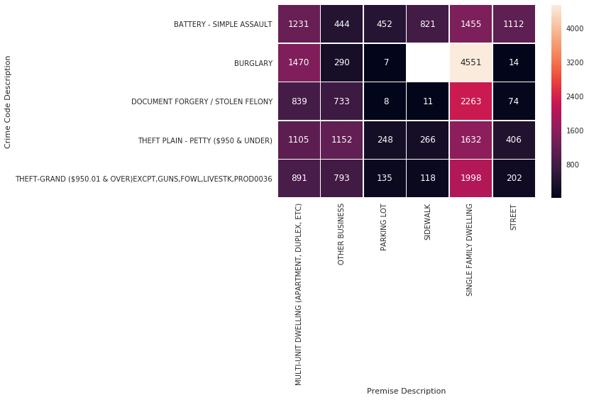
Excluding identity theft, we can observe the rest of the crime, more specifically, in a single dwelling house, since it is obvious from the diagram that it, along with identity theft is the top contender contributing the crime surge at 12PM.
- Burglary in single family dwelling. 12PM is usually a working hour, so home owners usually aren’t at home, hence an easy target for the criminals.
- Document forgery in single family dwelling. The same as identity theft, it is near impossible to know when document forgery occurs, so 12PM is the default rounding time for the crime.
- Grand theft and Petty theft in single family dwellings. Like the Burglary above, 12PM is usually a working hour, so home owners usually aren’t at home, hence an easy target for the criminals.
- Burglary in multi-unit dwellings also applicable to the logic above, most of the residence will be at work hence, an obvious target for crime.
4.7 Identity theft victim
In order for us to explore further, I filter the data with only identity theft crime, and create a subset with victim’s gender and age, which then dropped the null values.
identheftvic = crime[crime["Crime Code Description"] == "THEFT OF IDENTITY"]
identheftvic = identheftvic[["Victim Gender", "Victim Age"]]
identheftvic = identheftvic.dropna()
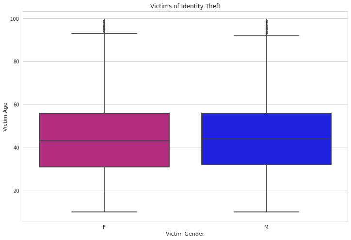
From the box plot above, we can observe that the distribution of the victims of identity theft are equally distributed regarding the age and gender of the victim. And this observation suggested that the criminals might be able to track their identity theft victim, regarding gender and age, in order to choose their next target without raising too much suspicion.
4.8 Monthly crime - without data from 2017 (dataset limit)
We could further observe the data by month better if we exclude the data from 2017, since the dataset got cut off in September 2017, hence the incomplete months in 2017.
I can do this by filtering out 2017 from the dataframe. And then create a new dataframe in order to visualize the intended data.
crimeno17 = crime.loc[crime["Year Occurred"].isin(range(2010, 2017))]
df = pd.DataFrame({
    'Month': list(crimeno17["Month Reported"].value_counts().index),
    'Crime Reported': list(crimeno17["Month Reported"].value_counts()),
    'Crime Occurred': list(crimeno17["Month Occurred"].value_counts())
})
monrepoccclean = df.set_index("Month").stack().reset_index().rename(columns={"level_1" : "Variable", 0 : "Crime"})
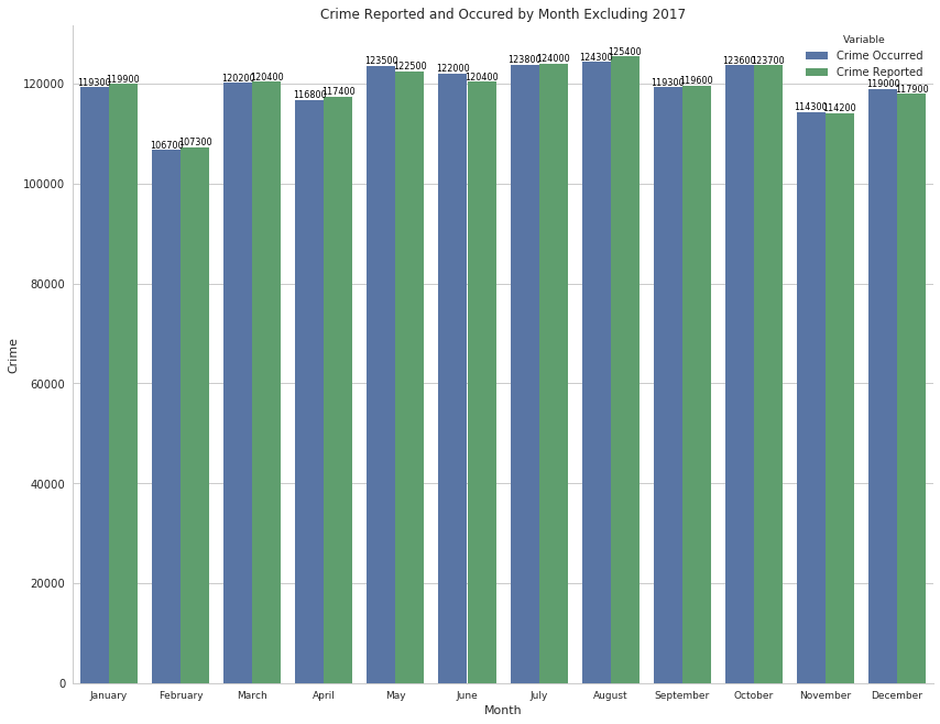
We can observe from the comparison bar graph above, with the exception of missing data from September to December 2017, the monthly distribution of crimes reported and occurrence is equal, which also proves our stance above that with months with 31 days having more than those with 30 or 28 days.
5 Modelling and Predictions
By using machine learning, we can predict type of crime, based on features such as day, month or premises.
In order to implement machine learning and build our model, we need to import a few libraries first.
from sklearn.linear_model import LinearRegression
from sklearn.model_selection import GridSearchCV
from sklearn.neighbors import KNeighborsClassifier
from sklearn.ensemble import RandomForestClassifier
from sklearn.metrics import classification_report
from sklearn.linear_model import LogisticRegression
from sklearn.model_selection import train_test_split
And them read the crime data once again, in case some of the manipulations remains and could potentially mess up the model. Then again, we reformat the date column to optimize the usability of the feature.
crime_df = pd.read_csv(path)
crime_df['Date Occurred'] = pd.to_datetime(
    crime_df['Date Occurred'].astype(str), errors='coerce')
crime_df['Date Occurred'] = pd.to_datetime(
    crime_df['Date Occurred'], format='%d/%m/%Y %H:%M:%S')
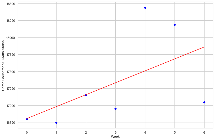
5.1 Linear Regression - Auto Stolen
| Target | Crime Code |
|---|---|
| Feature | Day, Month |
| Score | - |
Linear regression attempts to model the relationship between two variables by fitting a linear equation to observed data. One variable is considered to be an explanatory variable, and the other is considered to be a dependent variable. With the algorithm to be implement, we can directly apply it with the crime code feature and date or month to fit our linear regression model.
By Day
Weight coefficients: [[-74.93706294]] y-axis intercept: [10598.09090909]
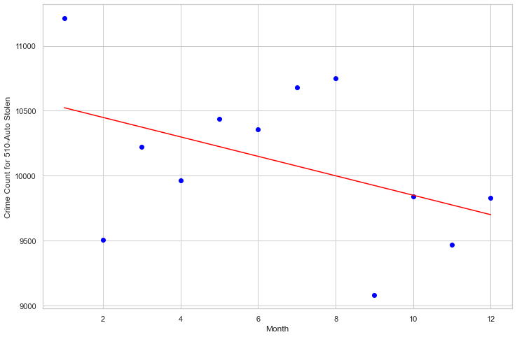
By Month
Weight coefficients: [[175.28571429]] y-axis intercept: [16807.28571429]
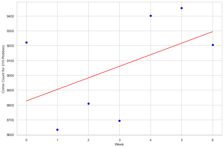
5.2 Linear Regression - Robbery
| Target | Crime Code |
|---|---|
| Feature | Day, Month |
| Score | - |
By Day
Weight coefficients: [[77.82142857]] y-axis intercept: [8826.82142857]
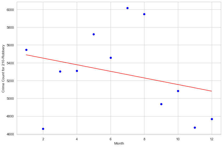
By Month
Weight coefficients: [[-37.13986014]] y-axis intercept: [5526.57575758]
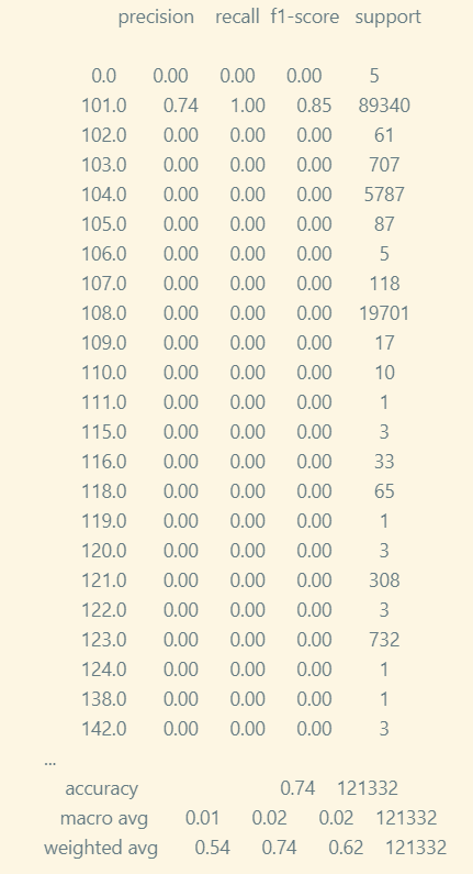
5.3 Logistic Regression Classifier
| Target | Crime Code |
|---|---|
| Feature | Premise Code |
| Score | 73% |
Logistic regression is a statistical method for predicting binary classes. The outcome or target variable contains only two possible classes. Which in this case the possible resulting classes are composed of Premise code 101: Street and 108: Parking Lot.
The logistic regression model concentrates on Crime Code 510 (Vehicle Stolen). With the help of Premise code (dwelling) as a predictor.
classifier = LogisticRegression()
The results are the following:
Training Data Score: 0.7375245881822877 Testing Data Score: 0.7327333267398543
5.4 Random Forest Classifier
| Target | Crime Code |
|---|---|
| Feature | Premise Code |
| Score | 89% |
A random forest is a meta estimator that fits a number of decision tree classifiers on various sub-samples of the dataset and uses averaging to improve the predictive accuracy and control over-fitting.
rf = RandomForestClassifier(n_estimators=20)
The resulting score, where n_estimators = 20 is the following:
Score = 0.8950565390828471
5.5 Grid Search Classifier
| Target | Crime Code |
|---|---|
| Feature | Premise Code |
| Score | 74% at {‘C’:1} |
We can pass a few predefined values for hyperparameters to the GridSearchCV function. We do this by defining a dictionary in which we mention a particular hyperparameter along with the values it can take. The “best” parameters that GridSearchCV identifies are technically the best that could be produced, but only by the parameters that you included in your parameter grid. Which in our case, the parameters are such that:
param_grid={‘C’: [1, 5, 10, 50]},
Fitting 5 folds for each of 4 candidates, totalling 20 fits
param_grid = {'C': [1, 5, 10, 50]}
grid = GridSearchCV(classifier, param_grid, verbose=3)
Which the results being:
Best Parameter = {‘C’: 1}
Best Score = 0.7363267731217805
5.6 K-Nearest Neighbor
| Target | Crime Code |
|---|---|
| Feature | Premise |
| Score | 73% (K=1000), 73% (K≥17) |
The KNN algorithm assumes that similar things exist in close proximity. In other words, similar things are near to each other. The KNN algorithm hinges on this assumption being true enough for the algorithm to be useful. KNN captures the idea of similarity (distance, proximity, or closeness) and calculating the distance between points on a graph.
For this algorithm, we separate the test into 2 sections, firstly with K = 1000, and the second with different value of K and compare them to find the point where the algorithm is stable enough, according to our data.
Testing with n_neighbors=1000
knn = KNeighborsClassifier(n_neighbors=1000)
Which provides the following results:
Test score = 0.7327333267398543
Train score = 0.7375245881822877
Testing with n_neighbors with different k value
for k in range(1, 20, 2):
    knn = KNeighborsClassifier(n_neighbors=k)
The results are the following:
k: 1, Train/Test Score: 1.000/0.603 k: 3, Train/Test Score: 0.785/0.691 k: 5, Train/Test Score: 0.760/0.709 k: 7, Train/Test Score: 0.750/0.718 k: 9, Train/Test Score: 0.745/0.723 k: 11, Train/Test Score: 0.743/0.726 k: 13, Train/Test Score: 0.742/0.728 k: 15, Train/Test Score: 0.741/0.729 k: 17, Train/Test Score: 0.740/0.730 k: 19, Train/Test Score: 0.740/0.730
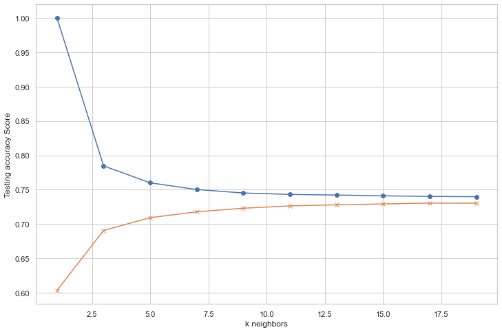
From the graph, we can observe that when K = 17, both the testing and the training score becomes stable.
6 Executive Summary
In order to take a closer look on the criminal activity from one of the most populated city in the USA to gain insights to the occurrences of the crime and it’s surrounding variables I chose the crime data from Los Angeles to be the focus of my analysis.
And by using analysis methodologies to explore insights from the data, several main points arises and has becomes clear:
- Saturday and Sunday are the 2 days that crimes are least likely to be reported, this is inarguably because, they are weekends. During weekends, people are less likely to be active, including both the criminal act and the duty of reporting the crime.
- Friday is the day that crime is most likely to occur. My analysis on this fact is that on Friday, more people will be out in the city and enjoying the night life, which mean, there will be more victims of petty crimes such as stealing or robbery for that day.
- We can see that months such as January or August, which have 31 days generally have more crimes than the ones with fewer days.
- We can see clearly that both of the graphs suggested that there is a surge of crimes occurring at 12PM.
- Mean of the victims are 35, and is supported by a median of 34.
- The sex of the victim are distributed as 51.4% being male, 46.9% being women, and 1.7% of other
- Hispanic/ Latin/ Mexican has been the crime victims of the most crime. While there are 7000 Korean crime victims and only 2000 Filipino crime victims.
- The top premise for crime committed is on the street and the runner-up is the single family dwelling.
- there are over 6 times more of the ongoing investigations than adult arrests.
- The most prominent crime is crime code 624, which is Battery and Simple Assault. And the follow up is crime code 510, which can be explain as Vehicles related crime.
Next I continue to explore more into some specific topics using methods and context surrounding the gathered data above as follows:
- Relationship between victim gender and crime type: Intimate partner sexual assault & Battery simple assault are the two crimes that women victims are more often are, which denotes the common occurrences of domestic violence that is still a common thing in the present, which is already more than a reason to fight for gender equality. And it is because there are more cars owned by males than females, that the crime such as burglary and vehicle stolen related crime has more male victim than women victims.
- Gun crime and correlated hours of occurrences: we can observe that firearm activities generally occur at night, between 7pm and before midnight, from both handgun and semi-automatic pistols.
- Premise and hour of crime: A prominent observation we can make is that the streets are generally less safe at night, and so is other crimes in the top 5 premises.
- Juvenile Arrest:
- The victim of the juvenile offenders tends to be between 10 to 20 years old.
- Battery and simple assault takes the lead to be the top type of crime juvenile arrest committed.
- There are nearly equal amounts of juvenile crimes committed on the street as in a single family dwelling.
- The crimes occur on weekdays since most juveniles are spending time with their family on the weekends.
- Juvenile crimes peaked between 12PM and 4 PM, which is also a school lunch hour, with the peak being at 3PM, as the time right after the school ends
- Safest and the most dangerous neighborhood: The population in 77th Street is dense and close in ratio of that with the Hollenbeck, the double in crime rate is surprisingly too significant. But this could also be missing the point of, what if these crimes were committed by someone not residing in the 77th Street.
- Crime surge at 12PM: Burglary in single family and multi unit dwelling —12PM is usually a working hour, so home owners usually aren’t at home, hence an easy target for the criminals.
- Identity theft victim sex and age: The victims of identity theft are equally distributed regarding the age and gender of the victim.
- Monthly crime without lack of 2017 data: With the exception of missing data from September to December 2017, the monthly distribution of crimes reported and occurrence is equal, which also proves our stance above that with months with 31 days having more than those with 30 or 28 days.
Lastly, by using machine learning, we can predict type of crime, based on features such as day, month or premises. Which the summary of each models are displayed as following:
| Model | Target | Feature | Score | Note |
|---|---|---|---|---|
| Linear Regression | Crime Code | Day, Month | - | Linear regression models the relationship between two variables by fitting a linear equation. And the two variables are crime code and premise. |
| Logistic Regression | Crime Code | Premise | 73% | The logistic regression model concentrates on Crime Code 510 (Vehicle Stolen). With the help of Premise code (dwelling) as a predictor. |
| Random Forest | Crime Code | Premise | 89% | Where n_estimators = 20 and it seems like this is the most optimal model. |
| Grid Search CV | Crime Code | Premise | 74% at {‘C’:1} | param_grid={‘C’: [1, 5, 10, 50]},Fitting 5 folds for each of 4 candidates, totalling 20 fits |
| K-Nearest Neighbor | Crime Code | Premise | 73% (K=1000), 73% (K≥17) | When K = 17, both the testing and the training score becomes stable. |